Month: November 2015

In the last part  we presented the major part of the UI, but we still hadn’t talked about the implementation of solving. In this post we will talk about how to actually solve non-linear equations both in theory and in implementation.

Non-linear circuits

Since last time, I took a pass at cleaning up the code and I decided to implement a few more components (inductors and diodes).   Inductors were relatively easy since it is still linear, but the diode presented more problems. Let’s go through the theory of non-linear solves.

We started in Part I laying out how to devise an equation per KCL node. Each equation becomes a row in the matrix and then we just solve a linear system to get the final values. That’s all good and fine, but it only works for linear components like resistors, inductors, capacitors and simple source terms like voltages and currents. For things like diodes and transistors which have crap loads of annoying non-linear exponential crap in them, we are kinda screwed. So, we must turn to nonlinear solving techniques, in particular Newton-Raphson iteration which root solves non linear equations by solving linear approximations and iterating. Let’s do a brief overview to see what we’ll need. Let’s suppose the ith equation

But since this is nonlinear. So using the taylor approximation we can write an approximation to the function as

where and is the Jacobian at the current iterate.
We still want the root to the approximation so we need to now solve

or specifically

Colloquially this is just a matrix equation . However, every Newton iteration we need to form a new A matrix. Thus given a current solution state we can go to a new one by following the steps:

1. Solve
2. Update the solution to be

On each time step we just repeat 1 and 2 as many times as needed for convergence given some norm. I just use check if is small for now. So to implement this, we need a way to form the matrix, a way to compute derivatives and a way to solve matrices.

Implementation

Building a matrix

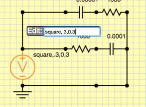
Conceptually, we need to form a matrix every time step and every Newton step. This requires two steps, identifying all the unknowns (which defines matrix dimensions), followed by determining the coefficients of the matrices. For various reasons (that probably are invalid and I will have to fix later) I thought it would be good to use separate objects for the solve and the UI. Thus, in the last segment we had a function that took “Symbol” objects and produced a final description like:

["R",["n1","n2"],1000]
["C",["n2","GND"],0.0001]
["V",["n1","GND"],"square,0.1,-1,1"]

We will go through the list and make “solver” objects now. It looks like this:

function createCircuitFromNetList(names,components){
    circuit=new Circuit();
    // Make a list of all the voltage nodes to graph
    namesToGraph=[]
    for(var n in names) namesToGraph.push(n);
    // Take visual components and turn them into simulation components
    for(var n in components){
        var node=components[n];
        switch(node[0]){
            case "R": circuit.addR(node[1][0],node[1][1],node[2]);break;
            case "C": circuit.addC(node[1][0],node[1][1],node[2]);break;
            case "V": circuit.addVoltage(node[1][0],node[1][1],node[2]);break;
            case "D": circuit.addD(node[1][0],node[1][1],node[2]);break;
            case "L": circuit.addI(node[1][0],node[1][1],node[2]);break;
        }
    }
    // solve and graph the circuit
    var foo=circuit.transient(3.0,.005,namesToGraph);
    graph(0,2,namesToGraph,foo);
}

Now essentially, we have connected up our UI part to our solver part. From here on out we are going to talk about the parts of the solver. It is possible to use those parts without a UI in a sense, so we basically have some compartmentalization!

Let’s look at what addR and addVoltage do because they are interesting:

Circuit.prototype.addVoltage=function(name1,name2,value){
    n1=this.allocNode(name1)
    n12=this.allocNode("sc"+this.num)
    n2=this.allocNode(name2)
    this.components.push(new Voltage(n1,n12,n2,value))
}
Circuit.prototype.addR=function(name1,name2,R){
    var n1=this.allocNode(name1)
    var n2=this.allocNode(name2);
    this.components.push(new Resistor(n1,n2,R))
}

The allocNode assigns that named node a number in the unknown vector. Once that is done, we make the component object using only the numbers. Each object knows how to contribute to the matrix and which values it contributes to. So in the example above we’d probably assign the matrix unknowns as [n1,n2,GND,sc3]. And remember these unknowns are going to actually be the delta in those values rather than the values themselves. Let’s look at how Resistor is implemented:

function Resistor(node1,node2,R){
    this.node1=node1
    this.node2=node2
    this.oneOverR=1.0/R
}
Resistor.prototype.matrix=function(dt, time, system, vPrev, xOld){
    system.addToMatrix(this.node1,this.node1,this.oneOverR);
    system.addToMatrix(this.node1,this.node2,-this.oneOverR);
    system.addToMatrix(this.node2,this.node1,-this.oneOverR);
    system.addToMatrix(this.node2,this.node2,this.oneOverR);
    system.addToB(this.node1,-vPrev[this.node1]*this.oneOverR+vPrev[this.node2]*this.oneOverR);
    system.addToB(this.node2,+vPrev[this.node1]*this.oneOverR-vPrev[this.node2]*this.oneOverR);
}

The constructor caches the nodes and the conductance (inverse of resistance). The matrix function is where all the magic happens. The function is called from the global build matrix function for all components. Several arguments are provided which are important to be able to add to the matrix. dt is the time step, time is the current time we are simulating at (good for voltage sources), system is an interface for adding values to the matrix, vPrev is the last newton iteration value ( in notation above). Why am I using v instead of x? Because I was stupid when I started writing this and thought everything would be a voltage, but clearly that can’t work. system provides two functions to use addToMatrix() and addToB that add stuff to the A matrix and the b right-hand-side, respectively. Everything we do to the matrix is opposite and equal and thus we always end up with a symmetric matrix, which is to be expected from a physical system. Also note that it is the linearity of the derivative that lets us differentiate the contribution to the full nodal equations for just the one component we are considering here.

Let’s dig into the math of the derivatives for a second. The contribution to the current of a resistor to a node will be I=V/R based on ohm’s law. So suppose we have a resistor for to . Then we have a contribution of on n1’s net current and net current. Differentiating with respect to each variable yields on each equation gives the Jacobian. These nodal equation derivatives only contribute to the rows corresponding to the KCL current and the only columns that are non-zero are the ones where the variable is n1 or n2. The derivative w.r.t. to either n1 or n2 gives 1/R (this is why we cached the conductance). Thus if this was the only equation our partial Jacobian matrix would look like

You can think of each component producing its own Jacobian matrix and just adding them all. Implementing the code like that would be very slow, so instead, we have this addToMatrix function do the same thing for us. On the right hand side we just evaluate the ohm’s law contributions with respect to the vPrev values. Thus our final system contribution from just the resistance in this particular case is
.
This is consistent with the code presented above.

Now that we’ve built the matrix for the resistor, let’s build it for the voltage source. The voltage has three matrix equations it contributes to. The two current equations for the nodes it is connected to and its own current which is unknown. From our example we have that where v is the voltage source that only depends on time. But we also have the unknown sc3 which contributes to the KCL current equation for n1 and GND. Thus this function

Voltage.prototype.matrix=function(dt,time,system,vprev,vold){
    // the constraint that the voltage from node1 to node2 is 5
    var v=5; // default to DC of constant 5 v
    if(this.type=="sin"){ 
    	v=(Math.sin(time*2*Math.PI/this.period)+1)*(this.max-this.min)*.5+this.min
    }
    // constrain the voltage
    system.addToMatrix(this.nodeCurrent,this.node1,1);
    system.addToMatrix(this.nodeCurrent,this.node2,-1);
    system.addToB(this.nodeCurrent,v-(vprev[this.node1]-vprev[this.node2]));
    // nodeCurrent is the current through the voltage source. it needs to be added to the KVL of node 1 and node2
    system.addToMatrix(this.node1,this.nodeCurrent,-1);
    system.addToMatrix(this.node2,this.nodeCurrent,1);
    system.addToB(this.node1,vprev[this.nodeCurrent]);
    system.addToB(this.node2,-vprev[this.nodeCurrent]);
}

yields on our example the matrix
.
It is somewhat weird that GND has all zeroes after my lecture about equal and opposite and symmetry. Well, the upshot is that GND is set to be zero, so we don’t let the matrix or right hand side get any contributions there (it is in the implementation of addToMatrix and addToB). At the end of the matrix construction we set the on-diagonal element for the gnd node row to be 1 which means that we enforce the equation gnd=0.

Each component has a similar implementation. Some are more complicated and need vOld as well (capacitors need to computer voltage derivatives). Since everybody has a definition, we have a simple buildMatrix function that makes the whole matrix:

Circuit.prototype.buildMatrix=function(vPrev,vOld,dt,time){
    var system=new System(this.num,this.ground);
    this.sys=system;
    for(var comp=0;comp<this.components.length;comp++){
        this.components[comp].matrix(dt,time,system,vPrev,vOld);
    }
}

Solving a matrix

Now we have constructed the matrix in our System object (which you need to look at the source code for). It basically consists of a array of arrays member called A and a array member consisting of b. We can solve the matrix equation using Gaussian elimination which we have just implemented in a straightforward way using partial pivoting (column swapping). Nothing exciting here, you can go look at wikipedia for more information on Gaussian elimination. That being said, using a dense matrix and gaussian elimination may not be the most efficient solver here. At least using a sparse LU or other optimized direct solver would be better. You could use LAPACK or SparseLU or whatever if you were in C/C++/Fortran. I am just in it for a quick and fast demo, but many opportunities for improvement are available which would be essential to make large circuits (1000’s of components) really efficient.

The Newton Solve

The full loop is implemented in transient() and it basically follows these steps:

function transient(maxTime,dt){
    vOld=vector(N,0); // N entries that are all zero
    vPrev=vector(N,0); // N entries that are all zero
    while(time<maxTime){
        vPrev.copyVector(vOld);
        for(var newton=0;newton<maxNewtonSteps;newton++){
            var matrix=buildMatrix(vPrev,vOld,dt,time);
            var difference=solve(matrix); /
            var maxDiff=difference.maxNorm();
            vPrev.addVector(difference)
            if(maxDiff < diffTolerance) break; // converged!
        }
        vOld=vPrev; // copy values
        time+=dt;
    }
    return vOld;
}

This is basically everything that is needed. There are several things that can go wrong. If you don’t specify a gnd, the solve will not work. If you make a loop of capacitors it probably won’t work. If you don’t have everything connected in a consistent way, it won’t work. There is very little error checking right now. It would be good to check if ground is connected. It would be good to check if the matrix is non-singular on every newton step.

A Diode

Before we finish let’s go through how the diode is implemented. This is a very important part because it is usually not talked about in simple circuit solvers that only do linear elements. A diode can be modeled by the Shockley equation that relates current to voltage

where is the saturation current of the diode, is the thermal voltage (26 mV at room temperature according to wikipedia) and varies between 1 and 2 to represent how ideal the diode is. Suppose we have nodal voltages n1 and n2, then we have . The derivatives with respect to n1 and n2 are
, respectively.

All this fun can be encoded into a component function that looks like this:

Diode.prototype.matrix=function(dt, time, system, vPrev, vOld){
	var n1=this.node1;
	var n2=this.node2;
	var denomInv=1./this.n*this.VT;
	var value=this.IS*(Math.exp((vPrev[n1]-vPrev[n2])*denomInv)-1)
	var deriv=this.IS*(Math.exp((vPrev[n1]-vPrev[n2])*denomInv))*denomInv;
	system.addToMatrix(this.node1,this.node1,deriv);
	system.addToMatrix(this.node1,this.node2,-deriv);
	system.addToMatrix(this.node2,this.node1,-deriv);
	system.addToMatrix(this.node2,this.node2,deriv);
	system.addToB(this.node1,-value);
	system.addToB(this.node2,value);
}

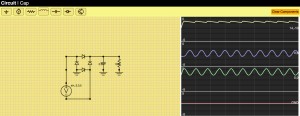
Using this we can now make a bridge rectifier circuit plus filter to turn AC into DC currents with minimal ripple.

Graphing

The transient() function populates arrays for each value it is requested to collect. These are then send to the graph() routine which is basically a html5 canvas draw routine that puts those on the graphs on the right. See the code for more details, nothing super exciting there. I would like to make the graphing selective and have the ability to graph some quantities on the same graph window, but this suffices for now. I would also like to extend the simulator to produce currents for every element as well. That will likely require some rework to how the matrices are created which will make the union find from the last post less important.

Try it yourself

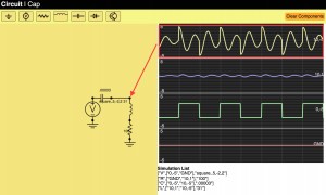
You can now try the program online at http://www.andyselle.com/circuit/.
There is still a lot more to do to make this an awesome circuit simulator, but it’s basically working. Yay! Here’s another example I did with some weird non-linear inductor behavior

 

Finally, I am picking up my long delayed circuit simulator. It’s been almost a year, so it is long overdue. There is no better time to do pointless educational programming projects than while vacationing. If you want to have a quick view of where we have gotten, see the youtube video at the bottom!

Anyways, in the part I we laid out the math for basic linear passives. In part II we made some of the UI for schematic capture. In this part we will advance the UI considerably. Below is a description of more problems we had to solve.

Adding components and adding wires

We now allow adding wires by clicking and dragging and we have a palette of components that can be added on demand. This was fairly uneventful. We also added “Backspace” and “r” as key options to delete and rotate the highlighted component.

Managing connections

Allowing users to connect components is probably the trickiest part of the UI. The basic idea I came up with is to always assume we are on a grid. Every pin will always lay on exactly aligned to the grid. If two components pins are on top of each other then they are considered connected. Let’s get into the implementation.

To do this, we need a data structure that can map from a location to which component(s) (or at least how many) are incident at the location. A major design constraint is that we want it to be sparse, that is we don’t want a dense array of the grid nodes, so we actually implement this as a hash table. For simplicity we just consider the key of the hash table to be the string xCoord+”,”+yCoord (so it is human readable). Probably it would be more efficient to do some bit fiddly stuff like ((x&0xffff)<<16)+(y &0xffff), but we are just making something simple, so I’m going to punt on that aspect of performance.

Each UI operation will call functions on every editable component called buildNet(recordNet,unionNet). recordNet and unionNet are functions that the component can call to record any pin’s grid coordinates and unionNet let’s the component consider two grid coordinates to be connected (i.e. a wire uses these). For a resistor the buildNet() function looks like this:

ResistorSymbol.prototype.buildNet=function(recordNet,unionNet)
{
   var n1=recordNet(this.objectToWorld(0,0));
   var n2=recordNet(this.objectToWorld(10,0));
   return ["R",[n1,n2],this.value];
}

This registers the two pins of the resistor and returns a full description of the resistor for the net list (more on that later). The WireSymbol not only registers new nodes but also unions the two nodes into one conceptual node:

WireSymbol.prototype.buildNet=function(netRecord,unionNet){
   var n0 = netRecord(
             this.objectToWorld(this.points[0][0],this.points[0][1]));
   var n1 = netRecord(
             this.objectToWorld(this.points[1][0],this.points[1][1]));
   unionNet(n0,n1);
}

What does netRecord do? Basically it makes grid location based name and puts it into a hash table with the key being the name and the value being [<xcoord>,<ycoord>,<numberOfComponentPinsIncident>,<parentSet>]. xcoord and ycoord are obvious, <numbertOfComponentPinsIncident> allows us to draw an open circle when there is 1 unconnected pin, and a solid circle when everything is connected. Each component pin that touches this grid node increments that value. Lastly, parentSet is the name of the parent set in which we are contained. This will be explained below in the union set finding. The result of the buildNet() function is we have a data structure the UI can query when it is drawing to make open or closed circles at the pin locations.

Creating the net list

Given a schematic, we would like to create a net list which is a description of what the components are and how they are connected. This is different than the schematic which has extraneous spatial information. For simulation we want a distilled description with only bare essentials needed for the simulator. In basic circuit analysis we use the lumped element model where any wire connections are assumed to be ideal. That means that any pins connected by wires become a single node. To accomplish this, we need to track connected components, so we will use a disjoint forest tree algorithm. For simplicity I am going to omit using the rank heuristic, but that would be easy to add to get the coveted inverse Ackermann function big-O performance. Remember the <parentSet> item in the node hash table discussed above. We start that equal to the key in the hash table. This means that the node is its own parent. Since everybody starts that way, everybody starts as a set of 1. Any unioning will change one of the parent entries to be the other. This implies trees and we can always find the effective name of the set by following parent links from a given node. To see this in action, consider this circuit where no unioning has been done:

If we union one of the wire’s two pins we get:

If we union the other wire we get:

This is all good and find, but we actually need to handle GND specially.Anything that unions with GND gets parent being GND. GND basically has ultimate priority over everybody. To do this, we have a special GND entry.

After doing unioning of GND with its pin, we get this.

Now remember how components returned a simplified description. Those are always done in terms of immediate names. They aren’t the final unioned set representative. For example we would get [“R”,[“0,0″,”5,0”],1000] rather than the canonical effective names [“R”,[“0,0″,”GND”],1000]. So before display them, we need to lookup the final name by traversing the parent tree (this is the findSet() algorithm for disjoint forests).

Once we’re done with all this business, we can print out components we are interested in with lumped and unioned node names as shown below:

This representation is perfect, because we can use it to create a circuit simulation structure that actually can solve the circuit.

Editing component values

One last but important part is that we need some way to edit resistances, capacitances and set parameters for voltage sources. We could get arbitrarily complex, so for now, I am going to keep it simple. Every component just stores a string, and I can put whatever I want there. For the voltage source I am going to use <wavetype=sin|square|triangle>,<period in s>,<voltsMin>,<voltsMax>. Then, whenever somebody double clicks on a component, they will get an edit box to change the parameters. I might want to have more first class parameters types in the future, but this will get me by, and it took 5 minutes to implement! See here:

Moving on

That’s probably enough for this time. I have made considerable progress on the simulator, and I will discuss how that was constructed in the next segment. To wet your appetite on how that works, take a look at this video of the simulator in action…